Showing posts with label GIS. Show all posts
Showing posts with label GIS. Show all posts
Sunday, September 20, 2015
Calculate Single Contour-Line from DEM with QGIS / GDAL
In QGIS:
- from menu: Raster / Extraction / Contour
- define output name path/to/output.shp
- alter GDAL call for single contour line at 900 m asl:
gdal_contour -fl 900 "path/to/dem_raster.asc" "path/to/output.shp"
- for removing small poplygons or lines add area or length field (attr table / field calc or vector / geometry / add geometry)
- query by length or area to deselect unwanted iso-lines
Finally, you can export the contours as KML and check it in Google Earth:

I downloaded my DEM-rasters (Nord-Tirol, Österreich) HERE
Read more »
- from menu: Raster / Extraction / Contour
- define output name path/to/output.shp
- alter GDAL call for single contour line at 900 m asl:
gdal_contour -fl 900 "path/to/dem_raster.asc" "path/to/output.shp"
- for removing small poplygons or lines add area or length field (attr table / field calc or vector / geometry / add geometry)
- query by length or area to deselect unwanted iso-lines
Finally, you can export the contours as KML and check it in Google Earth:

I downloaded my DEM-rasters (Nord-Tirol, Österreich) HERE
Make a KML-File from an OpenStreetMap Trail
Ever wished to use a trail on OSM on your GPS or smartphone? With this neat little R-Script this can easily be done. You'll just need to search OpenStreetMap for the ID of the trail (way), put this as argument to osmar::get_osm, convert to KML and you're good to go!


Read more »


# get OSM data
library(osmar)
library(maptools)

rotewandsteig <- get_osm(way(166274005), full = T)
sp_rotewandsteig <- as_sp(rotewandsteig, what = "lines")

# convert to KML
kmlLine(sp_rotewandsteig@lines[[1]], kmlfile = "rotewandsteig.kml",
        lwd = 3, col = "blue", name = "Rotewandsteig")

# view it
shell.exec("rotewandsteig.kml")
Custom Feature Edit Forms in QGIS with Auto-Filling Using PyQt
For anyone interested in the capabilities of customized feature edit forms in QGIS I'd like to reference the following GIS-Stackexchange posting: http://gis.stackexchange.com/questions/107090/auto-populate-field-as-concatenation-of-other-fields
Read more »
Quick GIS-Tip: Permanentely Sort Attribute Table by Attribute
Here's a short shell-script (I have C:\OSGeo4W64\bin\ on my PATH) for sorting GIS data, a sqlite-db in this case, and saving it in the newly created order to a file. The DB is sorted in ascending order by the attribute 'Name' and written to a file with the KML Driver.
Read more »
cd C:/Users/Kay/Documents/Web/Openlayers/Docs/Digitizing
ogr2ogr -sql "SELECT * FROM 'trails-db' ORDER BY Name ASC" -f "KML" trails.kml trails.sqlite
Use GDAL from R Console to Split Raster into Tiles

The screenshot to the left shows a raster in QGIS that was split into four parts with the below script.
## get filesnames (assuming the datasets were downloaded already.
## please see http://onlinetrickpdf.blogspot.co.at/2013/06/use-r-to-bulk-download-digital.html
## on how to download high-resolution DEMs)
setwd("D:/GIS_DataBase/DEM")
files <- dir(pattern = ".hgt")

## function for single file processing mind to replace the PATH to gdalinfo.exe!
## s = division applied to each side of raster, i.e. s = 2 gives 4 tiles, 3 gives 9, etc.
split_raster <- function(file, s = 2) {

    filename <- gsub(".hgt", "", file)
    gdalinfo_str <- paste0("\"C:/OSGeo4W64/bin/gdalinfo.exe\" ", file)

    # pick size of each side
    x <- as.numeric(gsub("[^0-9]", "", unlist(strsplit(system(gdalinfo_str, intern = T)[3], ", "))))[1]
    y <- as.numeric(gsub("[^0-9]", "", unlist(strsplit(system(gdalinfo_str, intern = T)[3], ", "))))[2]

    # t is nr. of iterations per side
    t <- s - 1
    for (i in 0:t) {
        for (j in 0:t) {
            # [-srcwin xoff yoff xsize ysize] src_dataset dst_dataset
            srcwin_str <- paste("-srcwin ", i * x/s, j * y/s, x/s, y/s)
            gdal_str <- paste0("\"C:/OSGeo4W64/bin/gdal_translate.exe\" ", srcwin_str, " ", "\"", file, "\" ", "\"", filename, "_", i, "_", j, ".tif\"")
            system(gdal_str)
        }
    }
}

## process all files and save to same directory
mapply(split_raster, files, 2)
Custom Google Hybrid Mapsource for MOBAC and GALILEO
For anyone having trouble with the shipped Google Hybrid mapsource, as I encountered them - here is a custom mapsource which worked for me. Save this as XML (under Win7) to ..
And for any Galileo user interested, I also add a custom mapsource:
Read more »
   Custom Google Hybrid
   10
   19
   png
   None
        http://mt{$serverpart}.google.com/vt/lyrs=y&x={$x}&y={$y}&z={$z}
  0 1
   #000000
And for any Galileo user interested, I also add a custom mapsource:
Google Hybrid
http://mt{$serverpart}.google.com/vt/lyrs=y&x={$x}&y={$y}&z={$z}
0 1
Programmatically Download CORINE Land Cover Seamless Vector Data with R
require(XML)

path_to_files <- "D:/GIS_DataBase/CorineLC/Seamless"
dir.create(path_to_files)
setwd(path_to_files)

doc <- htmlParse("http://www.eea.europa.eu/data-and-maps/data/clc-2006-vector-data-version-2")
urls <- xpathSApply(doc,'//*/a[contains(@href,".zip/at_download/file")]/@href')

# function to get zip file names
get_zip_name <- function(x) unlist(strsplit(x, "/"))[grep(".zip", unlist(strsplit(x, "/")))]

# function to plug into sapply
dl_urls <- function(x) try(download.file(x, get_zip_name(x), mode = "wb"))

# download all zip-files
sapply(urls, dl_urls)

# function for unzipping
try_unzip <- function(x) try(unzip(x))

# unzip all files in dir and delete them afterwards
sapply(list.files(pattern = "*.zip"), try_unzip)

# unlink(list.files(pattern = "*.zip"))
How to Integrate OpenStreetMap Nominatim Search into a Webpage or OpenLayers Map
Here' a concise example on how to integrate Nominatim search into a webpage:
http://jsfiddle.net/gimoya/yp8hmog7
And here's a live Openlayers example:
http://gimoya.bplaced.net/Openlayers/Bergfex/bergfex.html

Read more »
http://jsfiddle.net/gimoya/yp8hmog7
And here's a live Openlayers example:
http://gimoya.bplaced.net/Openlayers/Bergfex/bergfex.html

Use Case: Make Contour Lines for Google Earth with Spatial R

Displaying any Google Maps Content in Google Earth via Network-Links
This is a handy option for displaying Google Maps in Google Earth. This could be any of your own maps created in Google Maps, a route or whatever. One nice feature of GE's Network-Links is that if you or any other contributor of a Google map modifies it (in Google Maps), it will be refreshed also in Google Earth.To do so, just grab the link from Google Maps. Like this one for a route:
https://maps.google.at/maps?saddr=Tivoli+Stadion+Tirol,+Innsbruck&daddr=Haggen,+Sankt+Sigmund+im+Sellrain&hl=de&ll=47.227496,11.250687&spn=0.12007,0.338173&sll=47.230526,11.250825&sspn=0.120063,0.338173&geocode=FagR0QIdYR-uACGQHB8W0fIkjCkfsEUhQ2mdRzGQHB8W0fIkjA%3BFZhY0AId6CypACnvxXqyRz2dRzG6da9r3hgbNA&oq=hagge&t=h&dirflg=h&mra=ls&z=12
Then go to GE and choose "Add" from main menu and "Network-Link" from the submenu. Then paste the above link and append "&output=kml" to it. That's it!
Read more »
https://maps.google.at/maps?saddr=Tivoli+Stadion+Tirol,+Innsbruck&daddr=Haggen,+Sankt+Sigmund+im+Sellrain&hl=de&ll=47.227496,11.250687&spn=0.12007,0.338173&sll=47.230526,11.250825&sspn=0.120063,0.338173&geocode=FagR0QIdYR-uACGQHB8W0fIkjCkfsEUhQ2mdRzGQHB8W0fIkjA%3BFZhY0AId6CypACnvxXqyRz2dRzG6da9r3hgbNA&oq=hagge&t=h&dirflg=h&mra=ls&z=12
Then go to GE and choose "Add" from main menu and "Network-Link" from the submenu. Then paste the above link and append "&output=kml" to it. That's it!
QspatiaLite Use Case: Find Dominant Species and Species Count within Sampling Areas Using the QspatiaLite Plugin
This blogpost shows how to find the dominant species and species counts within sampling polygons. The Species-layer that I'll use here is comprised of overlapping polygons which represent the distribution of several species. The Regions-layer represents areas of interest over which we would like to calculate some measures like species count, dominant species and area occupied by the dominant species.
Since QGIS now makes import/export and querying of spatial data easy, we can use the spatiaLite engine to join the intersection of both layers to the region table and then aggregate this intersections by applying max- and count-function on each region. We'll also keep the identity and the area-value of the species with the largest intersecting area.
For the presented example I'll use
Regions, which is a polygon layer with a areas of interest
Species, which is a polygon layer with overlapping features, representing species
Do the calculation in 2 easy steps:
Import the layers to a spatiaLite DB with the Import function of the plugin (example data: HERE)
Run the query. For later use you can load this table to QGIS or export with the plugin's export button.
Addendum:
If you wish to calculate any other diversity measures, like Diversity- or Heterogenity-Indices, you might just run the below query (which actually is the subquery from above) and feed the resulting table to any statistic-software!
The output table will contain region's IDs, each intersecting species and the intersection area.
The intersection area, which is the species' area per polygon, is the metric that would be used for the calculation of diversity / heterogenity measures, etc. of regions!

I tested this on
QGIS 2.6 Brighton
with the QspatiaLite Plugin installed
Read more »
Since QGIS now makes import/export and querying of spatial data easy, we can use the spatiaLite engine to join the intersection of both layers to the region table and then aggregate this intersections by applying max- and count-function on each region. We'll also keep the identity and the area-value of the species with the largest intersecting area.
For the presented example I'll use
Do the calculation in 2 easy steps:
SELECT
  t.region AS region,
  t.species AS sp_dom,
  count(*) AS sp_number,
  max(t.sp_area) / 10000 AS sp_dom_area
  FROM (
      SELECT
          g.region AS region, s.species AS species,
          area(intersection(g.Geometry, s.Geometry)) AS sp_area
          FROM Regions AS g JOIN Sp_Distribution AS s
          ON INTERSECTS(g.Geometry, s.Geometry)
  ) AS t
GROUP BY t.region
ORDER BY t.region
Addendum:
If you wish to calculate any other diversity measures, like Diversity- or Heterogenity-Indices, you might just run the below query (which actually is the subquery from above) and feed the resulting table to any statistic-software!
The output table will contain region's IDs, each intersecting species and the intersection area.
The intersection area, which is the species' area per polygon, is the metric that would be used for the calculation of diversity / heterogenity measures, etc. of regions!
SELECT
  g.region AS regID,
  s.species AS sp,
  AREA(INTERSECTION(g.geometry, s.geometry)) AS sp_area
FROM Regions AS g JOIN Sp_Distribution AS s
ON INTERSECTS(g.Geometry,s.Geometry)
ORDER BY regID, sp_area ASC

I tested this on
Quick Tip for Austrian MOBAC Users: A Link to a Mapsource for Bergfex Topographic Map!
Here's a link to a Beanshell script enabling Bergfex topographic maps (OEK 50) as mapsource in MOBAC. With this mapsoursce and MOBAC you can create really nice offline topographic maps for Austria and use the created tiles for your special purposes.
Read more »
QspatiaLite Use Case: Query for Species Richness within Search-Radius
Following up my previous blogpost on using SpatiaLite for the calculation of diversity metrics from spatial data, I'll add this SQL-query which counts unique species-names from the intersection of species polygons and a circle-buffer around centroids of an input grid. The species number within the bufferarea are joined to a newly created grid. I use a subquery which grabs only those cells from the rectangular input grid, for which the condition that the buffer-area around the grid-cell's centroid covers the species unioned polygons at least to 80%.
Example data is HERE. You can use the shipped qml-stylefile for the newly generated grid. It labels three grid-cells with the species counts for illustration.
Import grid- and Sp_distr-layers with QspatiaLite Plugin
Run query and choose option "Create spatial table and load in QGIS", mind to set "geom" as geometry column

Read more »
select
    g1.PKUID as gID,
    count (distinct s.species) as sp_num_inbu,
    g1.Geometry AS geom
from (
 select g.*
 from(select Gunion(geometry) as geom
           from Sp_distr) as u, grid as g
 where area(intersection(buffer(centroid(g.geometry), 500), u.geom)) > pow(500, 2)*pi()*0.8
) as g1 join Sp_distr as s on intersects(buffer(centroid( g1.Geometry), 500), s.Geometry)
group by gID

Nice Species Distribution Maps with GBIF-Data in R
Here's an example of how to easily produce real nice distribution maps from GBIF-data in R with package maps...

Read more »

# go to gbif and download a csv file with the species you
# want (example data)
# ..in R first set working directory to your download directory..
data <- read.csv("occurrence-search-1316347695527.CSV",
        header = T, sep = ",")

str(data)
require(maps)
pdf("myr_germ.pdf")
map("world", resolution = 75)
points(data$Longitude, data$Latitude, col = 2, cex = 0.05)
text(-140, -50, "MYRICARIA\nGERMANICA")
dev.off()

# that's all there is to it..
Rasterize CORINE Landcover 2006 Seamless Vector Data with OGR-rasterize
Following up my latest postings (HERE & HERE) on Corine Landcover I'll share how to rasterize this data at a desired resolution with OGR rasterize:

Read more »
cd D:/GIS_DataBase/CorineLC/shps_app_and_extr/

# grab extracted and appended / merged file, created previously:
myfile=extr_and_app.dbf

name=${myfile%.dbf}

# rasterize y- and x-resolution = 50 map units:
gdal_rasterize -a code_06 -tr 50 50 -l $name $myfile D:/GIS_DataBase/CorineLC/shps_app_and_extr/clc_tirol_raster_50.tif
R GIS: Generalizer for KML Paths
I'm posting a recent project's spin-off, which is a custom line-generalizer which I used for huge KML-paths. Anyone with a less clumpsy approach?
Read more »
## line generalizing function: takes two vectors of with x/ycoords
## and return ids of x/y elements which distance to its next element
## is shorter than the average distance between consecutive vertices
## multiplied by 'fac'
check_dist <- function(x, y, fac) {
    dm <- as.matrix(dist(cbind(x, y)))

    ## supradiagonal holds distance from 1st to 2nd, 2nd to 3rd, etc. element
    d <- diag(dm[-1, -ncol(dm)])
    mean_dist <- mean(d)
    keep <- logical()

    ## allways keep first..
    keep[1] <- T
    for (i in 1:(length(x) - 2)) {
        keep[i + 1] <- (d[i] > mean_dist * fac)
        message(paste0("Distance from item ", i, " to item ", i + 1, " is: ", d[i]))
    }
    message(paste0("Treshold is: ", mean_dist * fac))
    cat("--\n")
    ## .. and always keep last
    keep[length(x)] <- T
    return(keep)
}

## Testing function check_dist:
x <- rnorm(5)
y <- rnorm(5)
(keep <- check_dist(x, y, 1.2))

plot(x, y)
lines(x[keep], y[keep], lwd = 4, col = "green")
lines(x, y, lwd = 1, col = "red")
text(x, y + 0.1, labels = c(1:length(x)))


## exclude vertices by generalization rule. coordinate-nodes with low number of vertices,
## segments with less than 'min_for_gen' vertices will not be simplified, in any case coordinates will be
## rounded to 5-th decimal place

generalize_kml_contour_node <- function(node, min_for_gen, fac) {

    require(XML)

    LineString <- xmlValue(node, trim = T)

    LineStrSplit <- strsplit(unlist(strsplit(LineString, "\\s")), ",")

    # filter out empty LineStrings which result from strsplit on '\\s'
    LineStrSplit <- LineStrSplit[sapply(LineStrSplit, length) > 0]

    # all 3 values are required, in case of error see for missing z-values:
    x <- round(as.numeric(sapply(LineStrSplit, "[[", 1, simplify = T)), 5)
    y <- round(as.numeric(sapply(LineStrSplit, "[[", 2, simplify = T)), 5)
    z <- round(as.numeric(sapply(LineStrSplit, "[[", 3, simplify = T)), 5)

    # for lines longer than 'min_for_gen' vertices, generalize LineStrings
    if (length(x) >= min_for_gen) {
        keep <- check_dist(x, y, fac)
        x <- x[keep]
        y <- y[keep]
        z <- z[keep]
        xmlValue(node) <- paste(paste(x, y, z, sep = ","), collapse = " ")

        # for all other cases, insert rounded values
    } else {
        xmlValue(node) <- paste(paste(x, y, z, sep = ","), collapse = " ")
    }
}

## mind to use the appropiate namespace definition: alternatively use:
## c(kml ='http://opengis.net/kml/2.2')
kml_generalize <- function(kml_file, min_for_gen, fac) {
    doc <- xmlInternalTreeParse(kml_file)
    nodes <- getNodeSet(doc, "//kml:LineString//kml:coordinates", c(kml = "http://earth.google.com/kml/2.0"))
    mapply(generalize_kml_contour_node, nodes, min_for_gen, fac)
    saveXML(doc, paste0(dirname(kml_file), "/simpl_", basename(kml_file)))
}

## get KML-files and generalize them
kml_file <- tempfile(fileext = ".kml")
download.file("http://dev.openlayers.org/releases/OpenLayers-2.13.1/examples/kml/lines.kml",
              kml_file, mode = "wb")
kml_generalize(kml_file, 5, 0.9)
shell.exec(kml_file)
shell.exec(paste0(dirname(kml_file), "/simpl_", basename(kml_file)))
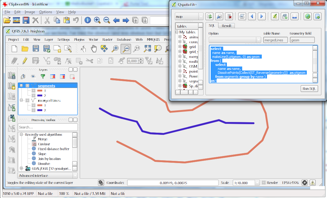
QspatiaLite Use Case: Connecting Lines
With QSpatiaLIte you can connect disjoint lines quite easily. With the below SQL you can allow for a grouping variable, in this case the field 'name' within the layer 'segments', by which the group vertices are collected and connected as lines! With this approach the vertices are connected in the order in which they were digitized and existing gaps are closed.


Read more »

select
  name as name,
  makeLine(t.ptgeom, 0) as geom
from (
     select
        name as name,
        DissolvePoints(Collect(ST_Reverse(geometry)))  as ptgeom
     from segments group by name )
as t
R GIS: Polygon Intersection with gIntersection{rgeos}
A short tutorial on doing intersections in R GIS. gIntersection{rgeos} will pick the polygons of the first submitted polygon contained within the second poylgon - this is done without cutting the polygon's edges which cross the clip source polygon. For the function that I use to download the example data, url_shp_to_spdf() please see HERE.

Read more »

library(rgeos)
library(dismo)

URLs <- c("http://gis.tirol.gv.at/ogd/umwelt/wasser/wis_gew_pl.zip",               # all water bodies in Tyrol
          "http://gis.tirol.gv.at/ogd/umwelt/wasser/wis_tseepeicher_pl.zip")       # only artificial..

y <- lapply(URLs, url_shp_to_spdf)
z <- unlist(unlist(y))
a <- getData('GADM', country = "AT", level = 2)

b <- a[a$NAME_2=="Innsbruck Land", ]                                               # political district's boundaries
c <- spTransform(b, z[[1]]@proj4string)                                            # (a ring polygon)
z1_c <- gIntersection(z[[1]], c, byid = TRUE)
z2_c <- gIntersection(z[[2]], c, byid = TRUE)

plot(c)
plot(z1_c, lwd = 5, border = "red", add = T)
plot(z2_c, lwd = 5, border = "green", add = T)
plot(z[[1]], border = "blue", add = T)              # I plot this on top, so it will be easier to identify
plot(z[[2]], border = "brown", add = T)
Line Slope Calculation in ArcGis 9.3 (using XTools)

You have a polyline, say a path, river, etc., and want to know average slope of each single line.
Approach:
Use z-values of nodes of polyline and calculate percentual slope by
(line-segment shape_length / z-Difference) * 100
Data:
A polyline (PL), a digital elevation model (DEM)
(1) Make point-shp-file from polyline nodes:
Xtools / Feature Conversions / Convert Feature to Points ->
check endpoints "from" & "to" (.. the nodes)
output = "PL_NODES"
(2) z-values at endpt_from & endpt_to:
Spatial Analyst / Extraction / Extract Values to Points ->
Input points = PL_NODES
Raster to extract = DEM
Output = PL_NODES_extr_DEM (...RASTERVALU = z-value)
(3) Get Difference in z-values for a segement (z at endpoint_from, z at endpoint_to):
Summary Statistics ->
Input Table = PL_NODE_extr_DHM,
Statistica Fields = RASTERVALU, Statistic Type = RANGE,
Case Field = Identifier for PL-Segments
output dbf = PL_NODE_dZ
(4) join PL_NODE_dZ to PL:
..use appropriate PL-IDs for joining
(5) add new field [slope_100] to PL:
..then use Field Calculator ->
slope_100 = 100* ( [PL_NODES_dZ.RANGE_RAST] / PL.SHAPE_LEN] )
Batch Downloading Zipped Shapefiles with R
Here's a function I use to download multiple zipped shapefiles from url and load them to the workspace:
Read more »
URLs <- c("http://gis.tirol.gv.at/ogd/umwelt/wasser/wis_gew_pl.zip",
          "http://gis.tirol.gv.at/ogd/umwelt/wasser/wis_tseepeicher_pl.zip")

url_shp_to_spdf <- function(URL) {

  require(rgdal)

  wd <- getwd()
  td <- tempdir()
  setwd(td)

  temp <- tempfile(fileext = ".zip")
  download.file(URL, temp)
  unzip(temp)

  shp <- dir(tempdir(), "*.shp$")
  lyr <- sub(".shp$", "", shp)
  y <- lapply(X = lyr, FUN = function(x) readOGR(dsn=shp, layer=lyr))
  names(y) <- lyr

  unlink(dir(td))
  setwd(wd)
  return(y)
  }

y <- lapply(URLs, url_shp_to_spdf)
z <- unlist(unlist(y))

# finally use it:
plot(z[[1]])
Subscribe to:
Posts (Atom)